TensorFlow Models
This chapter describes how to build a dynamic model with TensorFlow quickly.
Prerequisites:
- Python OOP (definition of classes & methods in Python, class inheritance, construction and destruction functions, using super() to call methods of the parent class, using __call__() to call an instance, etc.)
- Multilayer perceptrons, convolutional neural networks, recurrent neural networks and reinforcement learning (references given before each chapter).
Models & Layers
As mentioned in the last chapter, to improve the reusability of codes, we usually implement models as classes and use statements like y_pred() = model(X) to call the models. The structure of a model class is rather simple which basically includes __init__() (for construction and initialization) and call(input) (for model invocation) while you can also define your own methods if necessary. [1]
class MyModel(tf.keras.Model):
    def __init__(self):
        super().__init__()     # Use super(MyModel, self).__init__() under Python 2.
        # Add initialization code here (including layers to be used in the "call" method).

    def call(self, inputs):
        # Add model invocation code here (processing inputs and returning outputs).
        return output
Here our model inherits from tf.keras.Model. Keras is an advanced neural network API written in Python and is now supported by and built in official TensorFlow. One benefit of inheriting from tf.keras.Model is that we will be able to use its several methods and attributes like acquiring all variables in the model through the model.variables attribute after the class is instantiated, which saves us from indicating variables one by one explicitly.
Meanwhile, we introduce the concept of layers. Layers can be regarded as finer components encapsulating the computation procedures and variables compared with models. We can use layers to build up models quickly.
The simple linear model y_pred = tf.matmul(X, w) + b mentioned in the last chapter can be implemented through model classes:
import tensorflow as tf
tf.enable_eager_execution()

X = tf.constant([[1.0, 2.0, 3.0], [4.0, 5.0, 6.0]])
y = tf.constant([[10.0], [20.0]])


class Linear(tf.keras.Model):
    def __init__(self):
        super().__init__()
        self.dense = tf.keras.layers.Dense(units=1, kernel_initializer=tf.zeros_initializer(),
            bias_initializer=tf.zeros_initializer())

    def call(self, input):
        output = self.dense(input)
        return output


# The structure of the following codes is similar to the previous one.
model = Linear()
optimizer = tf.train.GradientDescentOptimizer(learning_rate=0.01)
for i in range(100):
    with tf.GradientTape() as tape:
        y_pred = model(X)      # Call the model.
        loss = tf.reduce_mean(tf.square(y_pred - y))
    grads = tape.gradient(loss, model.variables)
    optimizer.apply_gradients(grads_and_vars=zip(grads, model.variables))
print(model.variables)
Here we didn’t explicitly declare two variables W and b or write the linear transformation y_pred = tf.matmul(X, w) + b, but instead instantiated a densely-connected layer (tf.keras.layers.Dense) in the initialization and called this layer in the “call” method. The densely-connected layer encapsulates the output = activation(tf.matmul(input, kernel) + bias) linear transformation, the activation function, and two variables kernel and bias. This densely-connected layer would be equivalent to the aforementioned linear transformation if the activation function is not specified (i.e. activation(x) = x). By the way, the densely-connected layer may be the most frequent in our daily model coding.
Please refer to Custom Layers if you need to declare variables explicitly and customize operations.
| [1] | In Python classes, calling instances of the class myClass by such as myClass() is equivalent to myClass.__call__(). Here our model inherits from the parent class tf.keras.Model. This class includes the definition of __call__(), calling call() and also doing some internal keras operations. By inheriting from tf.keras.Model and overloading its call() method, we can add the codes for calling while keep the structure of keras, for details please refer to the __call__() part of the prerequisites in this chapter. |
A Basic Example: Multilayer Perceptrons (MLP)
Let’s begin with implementing a simple Multilayer Perceptron as an introduction of writing models in TensorFlow. Here we use the multilayer perceptron to classify the MNIST handwriting digit image dataset.
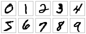
An image example of MNIST handwriting digits.
Before the main course, we implement a simple DataLoader class for loading the MNIST dataset.
class DataLoader():
    def __init__(self):
        mnist = tf.contrib.learn.datasets.load_dataset("mnist")
        self.train_data = mnist.train.images                                 # np.array [55000, 784].
        self.train_labels = np.asarray(mnist.train.labels, dtype=np.int32)   # np.array [55000] of int32.
        self.eval_data = mnist.test.images                                   # np.array [10000, 784].
        self.eval_labels = np.asarray(mnist.test.labels, dtype=np.int32)     # np.array [10000] of int32.

    def get_batch(self, batch_size):
        index = np.random.randint(0, np.shape(self.train_data)[0], batch_size)
        return self.train_data[index, :], self.train_labels[index]
The implementation of the multilayer perceptron model class is similar to the aforementioned linear model class except the former has more layers (as its name “multilayer” suggests) and introduces a nonlinear activation function (here ReLU function is used by the code activation=tf.nn.relu below). This model receives a vector (like a flattened 1*784 handwriting digit image here) and outputs a 10 dimensional signal representing the probability of this image being 0 to 9, respectively. Here we introduce a “predict” method which predicts the handwriting digits. It chooses the digit with the maximum likelihood as an output.
class MLP(tf.keras.Model):
    def __init__(self):
        super().__init__()
        self.dense1 = tf.keras.layers.Dense(units=100, activation=tf.nn.relu)
        self.dense2 = tf.keras.layers.Dense(units=10)

    def call(self, inputs):
        x = self.dense1(inputs)
        x = self.dense2(x)
        return x

    def predict(self, inputs):
        logits = self(inputs)
        return tf.argmax(logits, axis=-1)
Define some hyperparameters for the model:
num_batches = 1000
batch_size = 50
learning_rate = 0.001
Instantiate the model, the data loader class and the optimizer:
model = MLP()
data_loader = DataLoader()
optimizer = tf.train.AdamOptimizer(learning_rate=learning_rate)
And iterate the following steps:
- Randomly read a set of training data from DataLoader;
- Feed the data into the model to acquire its predictions;
- Compare the predictions with the correct answers to evaulate the loss function;
- Differentiate the loss function with respect to model parameters;
- Update the model parameters in order to minimize the loss.
The code implementation is as follows:
for batch_index in range(num_batches):
    X, y = data_loader.get_batch(batch_size)
    with tf.GradientTape() as tape:
        y_logit_pred = model(tf.convert_to_tensor(X))
        loss = tf.losses.sparse_softmax_cross_entropy(labels=y, logits=y_logit_pred)
        print("batch %d: loss %f" % (batch_index, loss.numpy()))
    grads = tape.gradient(loss, model.variables)
    optimizer.apply_gradients(grads_and_vars=zip(grads, model.variables))
Then, we will use the validation dataset to examine the performance of this model. To be specific, we will compare the predictions with the answers on the validation dateset, and output the ratio of correct predictions:
num_eval_samples = np.shape(data_loader.eval_labels)[0]
y_pred = model.predict(data_loader.eval_data).numpy()
print("test accuracy: %f" % (sum(y_pred == data_loader.eval_labels) / num_eval_samples))
Output:
test accuracy: 0.947900
Note that we can easily get an accuracy of 95% with even a simple model like this.
Convolutional Neural Networks (CNN)
The Convolutional Neural Network is an artificial neural network resembled as the animal visual system . It consists of one or more convolutional layers, pooling layers and dense layers. For detailed theories please refer to the Convolutional Neural Network chapter of the Machine Learning course by Professor Li Hongyi of National Taiwan University.
The specific implementation is as follows, which is very similar to MLP except some new convolutional layers and pooling layers.
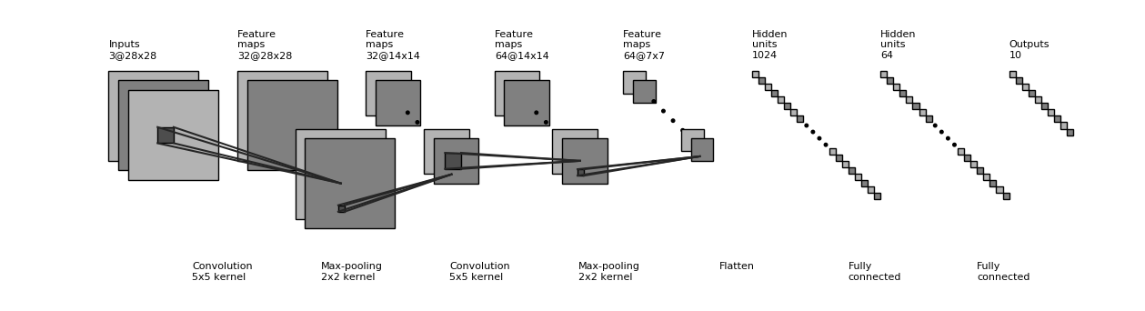
Figure of the CNN structure
class CNN(tf.keras.Model):
    def __init__(self):
        super().__init__()
        self.conv1 = tf.keras.layers.Conv2D(
            filters=32,             # Numbers of convolution kernels.
            kernel_size=[5, 5],     # Size of the receptive field.
            padding="same",         # Padding strategy.
            activation=tf.nn.relu   # Activation function.
        )
        self.pool1 = tf.keras.layers.MaxPool2D(pool_size=[2, 2], strides=2)
        self.conv2 = tf.keras.layers.Conv2D(
            filters=64,
            kernel_size=[5, 5],
            padding="same",
            activation=tf.nn.relu
        )
        self.pool2 = tf.keras.layers.MaxPool2D(pool_size=[2, 2], strides=2)
        self.flatten = tf.keras.layers.Reshape(target_shape=(7 * 7 * 64,))
        self.dense1 = tf.keras.layers.Dense(units=1024, activation=tf.nn.relu)
        self.dense2 = tf.keras.layers.Dense(units=10)

    def call(self, inputs):
        inputs = tf.reshape(inputs, [-1, 28, 28, 1])
        x = self.conv1(inputs)                  # [batch_size, 28, 28, 32].
        x = self.pool1(x)                       # [batch_size, 14, 14, 32].
        x = self.conv2(x)                       # [batch_size, 14, 14, 64].
        x = self.pool2(x)                       # [batch_size, 7, 7, 64].
        x = self.flatten(x)                     # [batch_size, 7 * 7 * 64].
        x = self.dense1(x)                      # [batch_size, 1024].
        x = self.dense2(x)                      # [batch_size, 10].
        return x

    def predict(self, inputs):
        logits = self(inputs)
        return tf.argmax(logits, axis=-1)
By substituting model = MLP() in the last chapter with model = CNN(), we get the following output:
test accuracy: 0.988100
We can see that there is a significant improvement of accuracy. In fact, the accuracy can be improved further by altering the network structure of the model (e.g. adding the Dropout layer to avoid overfitting).
Recurrent Neural Networks (RNN)
The Recurrent Neural Network is a kind of neural network suitable for processing sequential data, which is generally used for language modeling, text generation and machine translation, etc. For RNN theories, please refer to:
- Recurrent Neural Networks Tutorial, Part 1 – Introduction to RNNs.
- Recurrent Neural Network (part 1) and Recurrent Neural Network (part 2) from the Machine Learning course by Professor Li Hongyi of Taiwan University.
- The principles of LSTM: Understanding LSTM Networks.
- Generation of RNN sequences:[Graves2013].
Here we use RNN to generate a piece of Nietzsche style text. [2]
This task essentially predicts the probability distribution of the following alphabet of a given English text segment. For example, we have the following sentence:
I am a studen
This sentence (sequence) has 13 characters (including spaces) in total. Based on our experience, we can predict the following alphabet will probably be “t” when we read this sequence. We would like to build a model that receives num_batch sequences consisting of seq_length encoded characters and the input tensor with shape [num_batch, seq_length], and outputs the probability distribution of the following character with the dimension of num_chars (number of characters) and the shape [num_batch, num_chars]. We will sample from the probability distribution of the following character as a prediction and generate the second, third following characters step by step in order to complete the task of text generation.
First, we still implement a simple DataLoader class to read text and encode it in characters.
class DataLoader():
    def __init__(self):
        path = tf.keras.utils.get_file('nietzsche.txt',
            origin='https://s3.amazonaws.com/text-datasets/nietzsche.txt')
        with open(path, encoding='utf-8') as f:
            self.raw_text = f.read().lower()
        self.chars = sorted(list(set(self.raw_text)))
        self.char_indices = dict((c, i) for i, c in enumerate(self.chars))
        self.indices_char = dict((i, c) for i, c in enumerate(self.chars))
        self.text = [self.char_indices[c] for c in self.raw_text]

    def get_batch(self, seq_length, batch_size):
        seq = []
        next_char = []
        for i in range(batch_size):
            index = np.random.randint(0, len(self.text) - seq_length)
            seq.append(self.text[index:index+seq_length])
            next_char.append(self.text[index+seq_length])
        return np.array(seq), np.array(next_char)       # [num_batch, seq_length], [num_batch]
Then we implement the model. We instantiate a common BasicLSTMCell unit and a dense layer for linear transformation in the __init__ method. We first do an One-Hot operation on the sequence, i.e. transforming the code i into an n dimensional vector with the value 1 on the i-th position and value 0 elsewhere. Here n is the number of characters. The shape of the transformed sequence tensor is [num_batch, seq_length, num_chars]. After that, we will feed the sequences one by one into the RNN unit, i.e. feeding the state of the RNN unit state and sequences inputs[:, t, :] of the current time t into the RNN unit, and get the output of the current time output and the RNN unit state of the next time t+1. We take the last output of the RNN unit, transform it into num_chars dimensional one through a dense layer, and consider it as the model output.
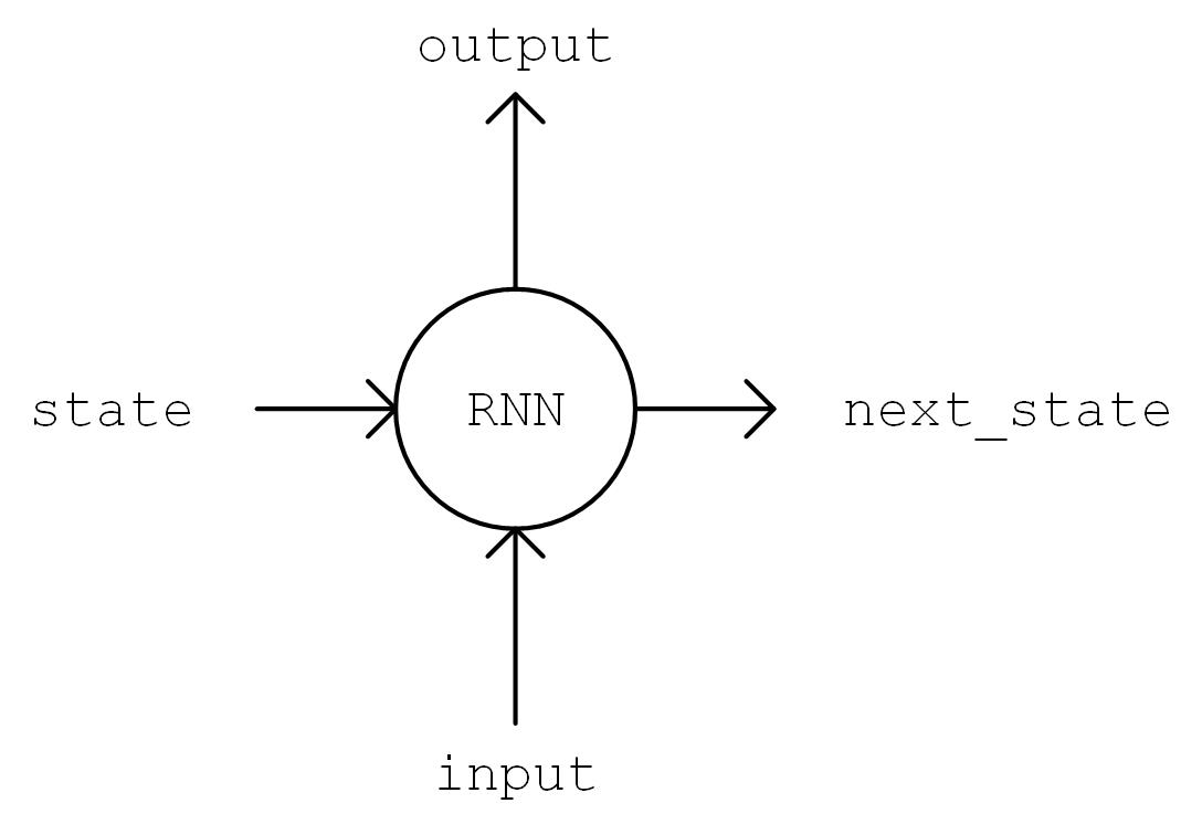
Figure of output, state = self.cell(inputs[:, t, :], state)
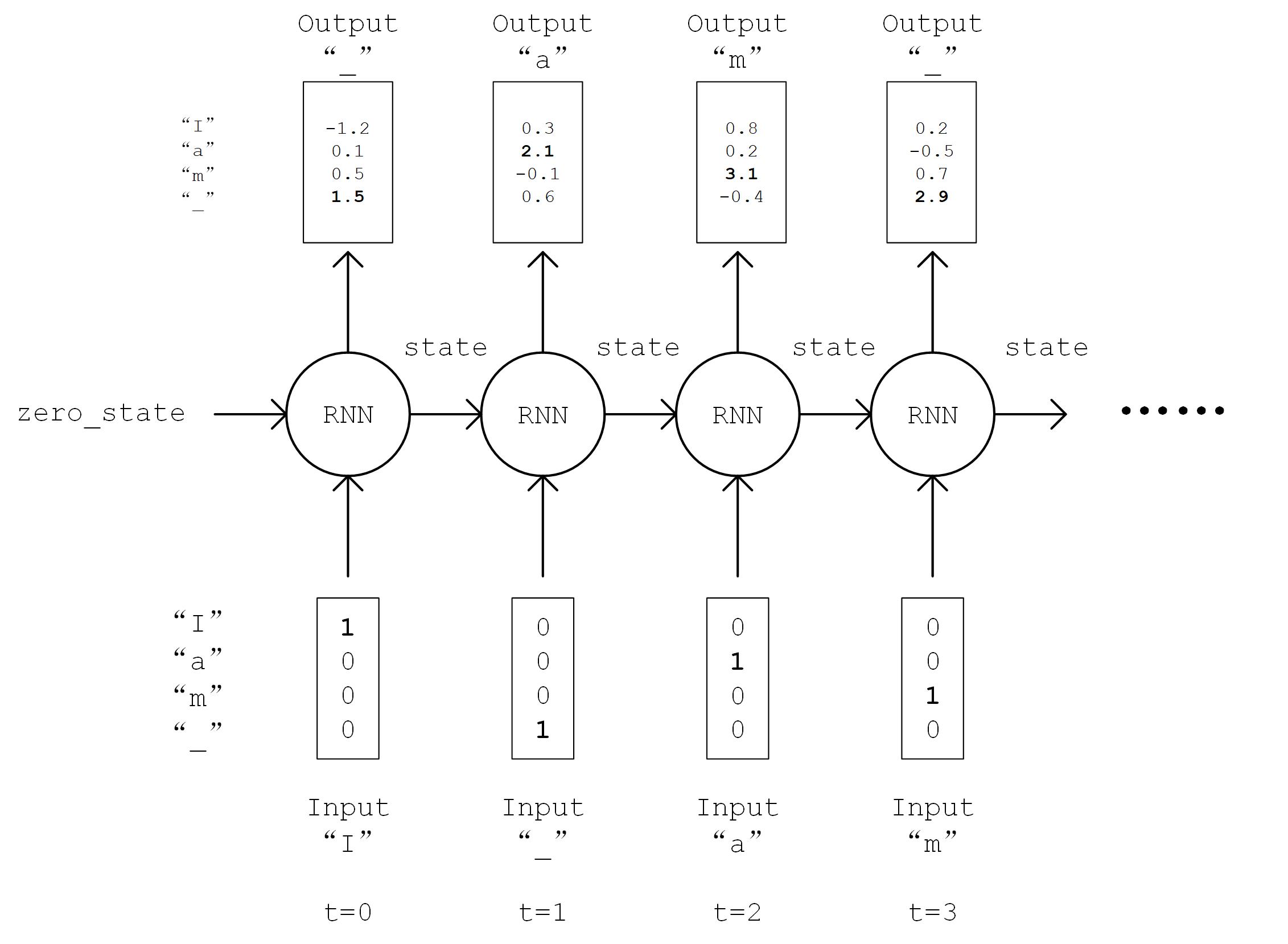
Figure of RNN process
The implementation is as follows:
class RNN(tf.keras.Model):
    def __init__(self, num_chars):
        super().__init__()
        self.num_chars = num_chars
        self.cell = tf.nn.rnn_cell.BasicLSTMCell(num_units=256)
        self.dense = tf.keras.layers.Dense(units=self.num_chars)

    def call(self, inputs):
        batch_size, seq_length = tf.shape(inputs)
        inputs = tf.one_hot(inputs, depth=self.num_chars)       # [batch_size, seq_length, num_chars]
        state = self.cell.zero_state(batch_size=batch_size, dtype=tf.float32)
        for t in range(seq_length.numpy()):
            output, state = self.cell(inputs[:, t, :], state)
        output = self.dense(output)
        return output
The training process is almost the same with the previous chapter, which we reiterate here:
- Randomly read a set of training data from DataLoader;
- Feed the data into the model to acquire its predictions;
- Compare the predictions with the correct answers to evaluate the loss function;
- Differentiate the loss function with respect to model parameters;
- Update the model parameters in order to minimize the loss.
    data_loader = DataLoader()
    model = RNN(len(data_loader.chars))
    optimizer = tf.train.AdamOptimizer(learning_rate=learning_rate)
    for batch_index in range(num_batches):
        X, y = data_loader.get_batch(seq_length, batch_size)
        with tf.GradientTape() as tape:
            y_logit_pred = model(X)
            loss = tf.losses.sparse_softmax_cross_entropy(labels=y, logits=y_logit_pred)
            print("batch %d: loss %f" % (batch_index, loss.numpy()))
        grads = tape.gradient(loss, model.variables)
        optimizer.apply_gradients(grads_and_vars=zip(grads, model.variables))
There is one thing we should notice about the process of text generation is that earlier we used the tf.argmax() function to regard the value with the maximum likelihood as the prediction. However, this method of prediction will be too rigid for text generation which also deprives the richness of the generated text. Thus, we use the np.random.choice() function for sampling based on the generated probability distribution by which even characters with small likelihood can still be possible to be sampled. Meanwhile we introduce the temperature parameter to control the shape of the distribution. Larger the value, flatter the distribution (smaller difference between the maximum and the minimum) and richer the generated text. Vice versa.
    def predict(self, inputs, temperature=1.):
        batch_size, _ = tf.shape(inputs)
        logits = self(inputs)
        prob = tf.nn.softmax(logits / temperature).numpy()
        return np.array([np.random.choice(self.num_chars, p=prob[i, :])
                         for i in range(batch_size.numpy())])
We can get the generated text by this step-by-step continuing prediction.
    X_, _ = data_loader.get_batch(seq_length, 1)
    for diversity in [0.2, 0.5, 1.0, 1.2]:
        X = X_
        print("diversity %f:" % diversity)
        for t in range(400):
            y_pred = model.predict(X, diversity)
            print(data_loader.indices_char[y_pred[0]], end='', flush=True)
            X = np.concatenate([X[:, 1:], np.expand_dims(y_pred, axis=1)], axis=-1)
The generated text is as follows:
diversity 0.200000:
conserted and conseive to the conterned to it is a self--and seast and the selfes as a seast the expecience and and and the self--and the sered is a the enderself and the sersed and as a the concertion of the series of the self in the self--and the serse and and the seried enes and seast and the sense and the eadure to the self and the present and as a to the self--and the seligious and the enders

diversity 0.500000:
can is reast to as a seligut and the complesed
has fool which the self as it is a the beasing and us immery and seese for entoured underself of the seless and the sired a mears and everyther to out every sone thes and reapres and seralise as a streed liees of the serse to pease the cersess of the selung the elie one of the were as we and man one were perser has persines and conceity of all self-el

diversity 1.000000:
entoles by
their lisevers de weltaale, arh pesylmered, and so jejurted count have foursies as is
descinty iamo; to semplization refold, we dancey or theicks-welf--atolitious on his
such which
here
oth idey of pire master, ie gerw their endwit in ids, is an trees constenved mase commars is leed mad decemshime to the mor the elige. the fedies (byun their ope wopperfitious--antile and the it as the f

diversity 1.200000:
cain, elvotidue, madehoublesily
inselfy!--ie the rads incults of to prusely le]enfes patuateded:.--a coud--theiritibaior "nrallysengleswout peessparify oonsgoscess teemind thenry ansken suprerial mus, cigitioum: 4reas. whouph: who
eved
arn inneves to sya" natorne. hag open reals whicame oderedte,[fingo is
zisternethta simalfule dereeg hesls lang-lyes thas quiin turjentimy; periaspedey tomm--whach
| [2] | The task and its implementation are referred to https://github.com/keras-team/keras/blob/master/examples/lstm_text_generation.py |
Deep Reinforcement Learning (DRL)
The Reinforcement Learning focuses on how to act in the environment in order to maximize the expected benefits. It becomes more powerful if combined with the deep learning technique. The recently famous AlphaGo is a typical application of the deep reinforcement learning. For its basic knowledge please refer to:
Here, we use the deep reinforcement learning to learn how to play CartPole. To be simple, our model needs to control the pole to keep it in a straight balance state.
The CartPole game
We use the CartPole game environment in the Gym Environment Library powered by OpenAI. Please refer to the official documentation and here for detailed installation steps and tutorials.
import gym

env = gym.make('CartPole-v1')       # Instantiate a game environment. The parameter is its name.
state = env.reset()                 # Initialize the environment and get its initial state.
while True:
    env.render()                    # Render the current frame.
    action = model.predict(state)   # Assume we have a trained model that can predict the action based on the current state.
    next_state, reward, done, info = env.step(action)   # Let the environment to execute the action, get the next state, the reward of the action, a flag whether the game is done, and extra information.
    if done:                        # Exit if the game is done.
        break
Therefore our task is to train a model that can predict good actions based on the current state. Roughly speaking, a good action should maximize the sum of rewards gained during the whole game process, which is also the target of reinforcement learning.
The following code shows how to use the Deep Q-Learning in deep reinforcement learning to train the model.
import tensorflow as tf
import numpy as np
import gym
import random
from collections import deque

tf.enable_eager_execution()
num_episodes = 500
num_exploration_episodes = 100
max_len_episode = 1000
batch_size = 32
learning_rate = 1e-3
gamma = 1.
initial_epsilon = 1.
final_epsilon = 0.01


# Q-network is used to fit Q function resemebled as the aforementioned multilayer perceptron. It inputs state and output Q-value under each action (2 dimensional under CartPole).
class QNetwork(tf.keras.Model):
    def __init__(self):
        super().__init__()
        self.dense1 = tf.keras.layers.Dense(units=24, activation=tf.nn.relu)
        self.dense2 = tf.keras.layers.Dense(units=24, activation=tf.nn.relu)
        self.dense3 = tf.keras.layers.Dense(units=2)

    def call(self, inputs):
        x = self.dense1(inputs)
        x = self.dense2(x)
        x = self.dense3(x)
        return x

    def predict(self, inputs):
        q_values = self(inputs)
        return tf.argmax(q_values, axis=-1)


env = gym.make('CartPole-v1')       # Instantiate a game environment. The parameter is its name.
model = QNetwork()
optimizer = tf.train.AdamOptimizer(learning_rate=learning_rate)
replay_buffer = deque(maxlen=10000)
epsilon = initial_epsilon
for episode_id in range(num_episodes):
    state = env.reset()             # Initialize the environment and get its initial state.
    epsilon = max(
        initial_epsilon * (num_exploration_episodes - episode_id) / num_exploration_episodes,
        final_epsilon)
    for t in range(max_len_episode):
        env.render()                # Render the current frame.
        if random.random() < epsilon:               # Epsilon-greedy exploration strategy.
            action = env.action_space.sample()      # Choose random action with the probability of epilson.
        else:
            action = model.predict(
                tf.constant(np.expand_dims(state, axis=0), dtype=tf.float32)).numpy()
            action = action[0]
        next_state, reward, done, info = env.step(action)               # Let the environment to execute the action, get the next state of the action, the reward of the action, whether the game is done and extra information.
        reward = -10. if done else reward                               # Give a large negative reward if the game is over.
        replay_buffer.append((state, action, reward, next_state, 1 if done else 0)) # Put the (state, action, reward, next_state) quad back into the experience replay pool.
        state = next_state

        if done:                                                        # Exit this round and enter the next episode if the game is over.
            print("episode %d, epsilon %f, score %d" % (episode_id, epsilon, t))
            break

        if len(replay_buffer) >= batch_size:
            # Randomly take a batch quad from the experience replay pool and transform them to NumPy array respectively.
            batch_state, batch_action, batch_reward, batch_next_state, batch_done = zip(
                *random.sample(replay_buffer, batch_size))
            batch_state, batch_reward, batch_next_state, batch_done = \
                [np.array(a, dtype=np.float32) for a in [batch_state, batch_reward, batch_next_state, batch_done]]
            batch_action = np.array(batch_action, dtype=np.int32)

            q_value = model(tf.constant(batch_next_state, dtype=tf.float32))
            y = batch_reward + (gamma * tf.reduce_max(q_value, axis=1)) * (1 - batch_done)  # Calculate y according to the method in the paper.
            with tf.GradientTape() as tape:
                loss = tf.losses.mean_squared_error(        # Minimize the distance between y and Q-value.
                    labels=y,
                    predictions=tf.reduce_sum(model(tf.constant(batch_state)) *
                                              tf.one_hot(batch_action, depth=2), axis=1)
                )
            grads = tape.gradient(loss, model.variables)
            optimizer.apply_gradients(grads_and_vars=zip(grads, model.variables))       # Calculate the gradient and update parameters.
Custom Layers *
Maybe you want to ask that what if these layers can’t satisfy my needs and I need to customize my own layers?
In fact, we can not only inherit from tf.keras.Model to write your own model class, but also inherit from tf.keras.layers.Layer to write your own layer.
class MyLayer(tf.keras.layers.Layer):
    def __init__(self):
        super().__init__()
        # Initialization.

    def build(self, input_shape):     # input_shape is a TensorFlow class object which provides the input shape.
        # Call this part when the layer is firstly used. Variables created here will have self-adapted shapes without specification from users. They can also be created in __init__ part if their shapes are already determined.
        self.variable_0 = self.add_variable(...)
        self.variable_1 = self.add_variable(...)

    def call(self, input):
        # Model calling (process inputs and return outputs).
        return output
For example, if we want to implement a dense layer in the first section of this chapter with a specified output dimension of 1, we can write as below, creating two variables in the build method and do operations on them:
class LinearLayer(tf.keras.layers.Layer):
    def __init__(self):
        super().__init__()

    def build(self, input_shape):     # Here input_shape is a TensorShape.
        self.w = self.add_variable(name='w',
            shape=[input_shape[-1], 1], initializer=tf.zeros_initializer())
        self.b = self.add_variable(name='b',
            shape=[1], initializer=tf.zeros_initializer())

    def call(self, X):
        y_pred = tf.matmul(X, self.w) + self.b
        return y_pred
With the same way, we can call our custom layers LinearLayer:
class Linear(tf.keras.Model):
    def __init__(self):
        super().__init__()
        self.layer = LinearLayer()

    def call(self, input):
        output = self.layer(input)
        return output
Graph Execution Mode *
In fact, these models above will be compatible with both Eager Execution mode and Graph Execution mode if we write them more carefully [3]. Please notice, model(input_tensor) is only needed to run once for building a graph under Graph Execution mode.
For example, we can also call the linear model built in the first section of this chapter and do linear regression by the following codes:
    model = Linear()
    optimizer = tf.train.GradientDescentOptimizer(learning_rate=0.01)
    X_placeholder = tf.placeholder(name='X', shape=[None, 3], dtype=tf.float32)
    y_placeholder = tf.placeholder(name='y', shape=[None, 1], dtype=tf.float32)
    y_pred = model(X_placeholder)
    loss = tf.reduce_mean(tf.square(y_pred - y_placeholder))
    train_op = optimizer.minimize(loss)
    with tf.Session() as sess:
        sess.run(tf.global_variables_initializer())
        for i in range(100):
            sess.run(train_op, feed_dict={X_placeholder: X, y_placeholder: y})
        print(sess.run(model.variables))
| [3] | In addition to the RNN model implemented in this chapter, we get the length of seq_length dynamically under Eager Execution, which enables us to easily control the expanding length of RNN dynamically, which is not supported by Graph Execution. In order to reach the same effect, we need to fix the length of seq_length or use tf.nn.dynamic_rnn instead (Documentation). |
| [LeCun1998] |
|
| [Graves2013] | Graves, Alex. “Generating Sequences With Recurrent Neural Networks.” ArXiv:1308.0850 [Cs], August 4, 2013. http://arxiv.org/abs/1308.0850. |
| [Mnih2013] | Mnih, Volodymyr, Koray Kavukcuoglu, David Silver, Alex Graves, Ioannis Antonoglou, Daan Wierstra, and Martin Riedmiller. “Playing Atari with Deep Reinforcement Learning.” ArXiv:1312.5602 [Cs], December 19, 2013. http://arxiv.org/abs/1312.5602. |