TensorFlow Basic
This chapter describes basic operations in TensorFlow.
Prerequisites:
- Basic Python operations (assignment, branch & loop statement, library import)
- ‘With’ statement in Python
- NumPy , a common library for scientific computation, important for TensorFlow
- Vectors & Matrices operations (matrix addition & subtraction, matrix multiplication with vectors & matrices, matrix transpose, etc., Quiz:
 )
) - Derivatives of functions , derivatives of multivariable functions (Quiz:
 )
) - Linear regression;
- Gradient descent that searches local minima of a function
TensorFlow 1+1
TensorFlow can be simply regarded as a library of scientific calculation (like Numpy in Python). Here we calculate  and
and  as our first example.
import tensorflow as tf
tf.enable_eager_execution()

a = tf.constant(1)
b = tf.constant(1)
c = tf.add(a, b)    # The expression c = a + b is equivalent.

print(c)

A = tf.constant([[1, 2], [3, 4]])
B = tf.constant([[5, 6], [7, 8]])
C = tf.matmul(A, B)

print(C)
Output:
tf.Tensor(2, shape=(), dtype=int32)
tf.Tensor(
[[19 22]
[43 50]], shape=(2, 2), dtype=int32)
The code above declares four tensors named a, b, A and B. It also invokes two operations tf.add() and tf.matmul() which respectively do addition and matrix multiplication on tensors. Operation results are immediately stored in the tensors c and C. Shape and dtype are two major attributes of a tensor. Here a, b and c are scalars with null shape and int32 dtype, while A, B, C are 2-by-2 matrices with (2, 2) shape and int32 dtype.
In machine learning, it’s common to differentiate functions. TensorFlow provides us with the powerful Automatic Differentiation Mechanism for differentiation. The following codes show how to utilize tf.GradientTape() to get the slope of  at
at  .
.
import tensorflow as tf
tf.enable_eager_execution()

x = tf.get_variable('x', shape=[1], initializer=tf.constant_initializer(3.))
with tf.GradientTape() as tape:     # All steps in the context of tf.GradientTape() are recorded for differentiation.
    y = tf.square(x)
y_grad = tape.gradient(y, x)        # Differentiate y with respect to x.
print([y.numpy(), y_grad.numpy()])
Output:
[array([9.], dtype=float32), array([6.], dtype=float32)]
Here x is a variable initialized to 3, declared by tf.get_variable(). Like common tensors, variables also have shape and dtype attributes, but require an initialization. We can assign an initializer to tf.get_variable() by setting the Initializer parameter. Here we use tf.constant_initializer(3.) to initialize the variable x to 3. with a float32 dtype. [1]. An important difference between variables and common tensors is that a function can be differentiated by variables, not by tensors, using the automatic differentiation mechanism by default. Therefore variables are usually used as parameters defined in machine learning models. tf.GraidentTape() is a recorder of automatic differentiation which records all variables and steps of calculation automatically. In the previous example, the variable x and the calculation step y = tf.square(x) are recorded automatically, thus the derivative of the tensor y with respect to x can be obtained through y_grad = tape.gradient(y, x).
In machine learning, calculating the derivatives of a multivariable function, a vector or a matrix is a more common case, which is a piece cake for TensorFlow. The following codes show how to utilize tf.GradientTape() to differentiate  with respect to
  and
and  at
at  .
.
X = tf.constant([[1., 2.], [3., 4.]])
y = tf.constant([[1.], [2.]])
w = tf.get_variable('w', shape=[2, 1], initializer=tf.constant_initializer([[1.], [2.]]))
b = tf.get_variable('b', shape=[1], initializer=tf.constant_initializer([1.]))
with tf.GradientTape() as tape:
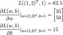
L = 0.5 * tf.reduce_sum(tf.square(tf.matmul(X, w) + b - y))
w_grad, b_grad = tape.gradient(L, [w, b]) # Differentiate L with respect to w and b.
print([L.numpy(), w_grad.numpy(), b_grad.numpy()])
Output:
[62.5, array([[35.],
   [50.]], dtype=float32), array([15.], dtype=float32)]
Here the operation tf.square() squares every element in the input tensor without altering its shape. The operation tf.reduce_sum() outputs the sum of all elements in the input tensor with a null shape (the dimensions of the summation can be indicated by the axis parameter, while all elements are summed up if not specified). TensorFlow contains a large number of tensor operation APIs including mathematical operations, tensor shape operations (like tf.reshape()), slicing and concatenation (like tf.concat()), etc. You can heck TensorFlow official API documentation [2] for further information.
As we can see from the output, TensorFlow helps us figure out that
A Basic Example: Linear Regression
Let’s consider a practical problem. The house prices of a city between 2013 and 2017 are given by the following table:
| Year | 2013 | 2014 | 2015 | 2016 | 2017 |
| Price | 12000 | 14000 | 15000 | 16500 | 17500 |
Now we want to do linear regression on the given data, i.e. using the linear model  to fit the data, where
 a and b are unknown parameters.
First, we define and normalize the data.
import numpy as np

X_raw = np.array([2013, 2014, 2015, 2016, 2017], dtype=np.float32)
y_raw = np.array([12000, 14000, 15000, 16500, 17500], dtype=np.float32)

X = (X_raw - X_raw.min()) / (X_raw.max() - X_raw.min())
y = (y_raw - y_raw.min()) / (y_raw.max() - y_raw.min())
Then, we use gradient descent to evaluate these two parameters a and b in the linear model [3].
Recalling from the fundamentals of machine learning, for searching local minima of a multivariable function  , we use gradient descent which taking the following steps:
Initialize the argument to
 and have
Iterate the following steps repeatedly till the convergence criteria is met:
- Find the gradient of the function with respect to the parameter

- Update the parameter
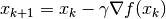 where
where  is the learning rate (like the step size of the gradient descent)
- Find the gradient of the function
Next we focus on how to implement gradient descent in order to solve the linear regression  .
.
NumPy
The implementation of machine learning models is not a patent of TensorFlow. In fact, even most common scientific calculators or tools can solve simple models. Here, we use Numpy, a general library for scientific computation, to implement gradient descent. Numpy supports multidimensional arrays to represent vectors, matrices and tensors with more dimensions. Meanwhile, it also supports lots of operations on multidimensional arrays (e.g. np.dot() calculates the inner products and np.sum() adds up all the elements). In this way Numpy is somewhat like MATLAB. In the following codes, we evaluate the partial derivatives of loss function with respect to the parameters a and b manually [4], and then iterate by gradient descent to acquire the value of a and b eventually.
a, b = 0, 0

num_epoch = 10000
learning_rate = 1e-3
for e in range(num_epoch):
    # Calculate the gradient of the loss function with respect to arguments (model parameters) manually.
    y_pred = a * X + b
    grad_a, grad_b = (y_pred - y).dot(X), (y_pred - y).sum()

    # Update parameters.
    a, b = a - learning_rate * grad_a, b - learning_rate * grad_b

print(a, b)
However, you may have noticed that there are several pain points using common libraries for scientific computation to implement machine learning models:
- It’s often inevitable to differentiate functions manually. Simple ones may be fine, however the more complex ones (especially commonly appeared in deep learning models) are another story. Manual differentiation may be painful, even infeasible in the latter cases.
- It’s also often inevitable to update parameters based on the gradients manually. Manual update is still easy here because the gradient descent is a rather basic method while it’s not going to be easy anymore if we apply a more complex approach to update parameters (like Adam or Adagrad).
However, the appearance of TensorFlow eliminates these pain points to a large extent, granting users convenience for implementing machine learning models.
TensorFlow
The Eager Execution Mode of TensorFlow [5] have very similar operations as the above-mentioned Numpy. In addition, it also provides us with a series of critical functions for deep learning such as faster operation speed (need support from GPU), automatic differentiation and optimizers, etc. We will show how to do linear regression using Tensorflow. You may notice that its code structure is similar to the one of Numpy. Here we delegates TensorFlow to do two important jobs:
- Using
tape.gradient(ys, xs)to get the gradients automatically; - Using
optimizer.apply_gradients(grads_and_vars)to update parameters automatically.
X = tf.constant(X)
y = tf.constant(y)

a = tf.get_variable('a', dtype=tf.float32, shape=[], initializer=tf.zeros_initializer)
b = tf.get_variable('b', dtype=tf.float32, shape=[], initializer=tf.zeros_initializer)
variables = [a, b]

num_epoch = 10000
optimizer = tf.train.GradientDescentOptimizer(learning_rate=1e-3)
for e in range(num_epoch):
    # Use tf.GradientTape() to record the gradient info of the loss function
    with tf.GradientTape() as tape:
        y_pred = a * X + b
        loss = 0.5 * tf.reduce_sum(tf.square(y_pred - y))
    # TensorFlow calculates the gradients of the loss function with respect to each argument (model paramter) automatically.
    grads = tape.gradient(loss, variables)
    # TensorFlow updates parameters automatically based on gradients.
    optimizer.apply_gradients(grads_and_vars=zip(grads, variables))
Here, we use the aforementioned approach to calculate the partial derivatives of the loss function with respect to each parameter, while we also use tf.train.GradientDescentOptimizer(learning_rate=1e-3) to declare an optimizer for graident descent with a learning rate of 1e-3. The optimizer can help us update parameters based on the result of differentiation in order to minimize a specific loss function by calling its apply_gradients() interface.
Note that, for calling optimizer.apply_gradients() to update model parameters, we need to provide it with parameters grads_and_vars, i.e. the variables to be updated (like variables in the aforementioned codes). To be specific, a Python list has to be passed, whose every element is a (partial derivative with respect to a variable, this variable) pair. For instance, [(grad_w, w), (grad_b, b)] is passed here. By executing grads = tape.gradient(loss, variables) we get partial derivatives of the loss function with respect to each variable recorded in tape, i.e. grads = [grad_w, grad_b]. Then we use zip() in Python to pair the elements in grads = [grad_w, grad_b] and vars = [w, b] together respectively so as to get the required parameters.
In practice, we usually build much more complex models rather the linear model y_pred = tf.matmul(X, w) + b here which can be simply written in a single line. Therefore, we often write a model class and call it by y_pred = model(X) when needed. The following chapter elaborates writing model classes.
| [1] | We can add a decimal point after an integer to make it become a floating point number in Python. E.g. 3. represents the floating point number 3.0. |
| [2] | Mainly refer to Tensor Transformations and Math. Note that the tensor operation API of TensorFlow is very similar to Numpy, thus one can get started on TensorFlow rather quickly if knowing about the latter. |
| [3] | In fact there is an analytic solution for the linear regression. We use gradient descent here just for showing you how TensorFlow works. |
| [4] | The loss function here is the mean square error 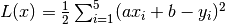 whose partial derivatives with respect to whose partial derivatives with respect to a and b are 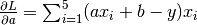 and and 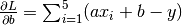 . . |
| [5] | The opposite of Eager Execution is Graph Execution that TensorFlow adopts before version 1.8 in Mar 2018. This handbook is mainly written for Eager Execution aiming at fast iterative development, however the basic usage of Graph Execution is also attached in the appendices in case of reference. |