TensorFlow Extensions
This chapter introduces some of the most commonly used TensorFlow extensions. Although these features are not “must”, they make the process of model training and calling more convenient.
Prerequisites:
- Python serialization module Pickle (not required)
- Python special function parameters **kwargs (not required)
Checkpoint: Saving and Restoring Variables
Usually, we hope to save the trained parameters (variables) after the model training is completed. By loading the model and parameters when you need model, you can get the trained model directly. Perhaps the first thing you think of is to store model.variables with the Python serialization module pickle. But unfortunately, TensorFlow’s variable type ResourceVariable cannot be serialized.
Fortunately, TensorFlow provides a powerful variable saving and restoring class tf.train.Checkpoint , which can save and restore all objects in the TensorFlow containing the Checkpointable State by save() and restore() methods. Specifically, tf.train.Optimizer implementations, tf.Variable, tf.keras.Layer implementations or tf.keras.Model implementations can all be saved. Its usage is very simple, we first declare a Checkpoint:
checkpoint = tf.train.Checkpoint(model=model)
Here the initialization parameter passed to tf.train.Checkpoint() is special, it is a **kwargs. Specifically, it is a series of key-value pairs, and the keys can be taken at will, and the values are objects that need to be saved. For example, if we want to save a model instance model that inherits tf.keras.Model and an optimizer optimizer that inherits tf.train.Optimizer, we can write:
checkpoint = tf.train.Checkpoint(myAwesomeModel=model, myAwesomeOptimizer=optimizer)
Here myAwesomeModel is any key we take to save the model model. Note that we will also use this key when restoring variables.
Next, when the trained model needs to be saved, use:
checkpoint.save(save_path_with_prefix)
is fine. save_path_with_prefix is the directory and prefix of the saved file. For example, if you create a folder named “save” in the source directory and call checkpoint.save('./save/model.ckpt') once, we can find three files in the directory named checkpoint, model.ckpt-1.index, and model.ckpt-1.data-00000-of-00001, which record variable information. The checkpoint.save() method can be run multiple times. Each time we will get an .index file and a .data file. The serial number increase gradually.
When you need to reload previously saved parameters for models elsewhere, you need to instantiate a checkpoint again, while keeping the keys consistent. Then call the restore method of checkpoint. Just like this:
model_to_be_restored = MyModel()                                        # The same model of the parameter to be restored
checkpoint = tf.train.Checkpoint(myAwesomeModel=model_to_be_restored)   # The key remains as "myAwesomeModel"
checkpoint.restore(save_path_with_prefix_and_index)
Then the model variables are restored. save_path_with_prefix_and_index is the directory + prefix + number of the previously saved file. For example, calling checkpoint.restore('./save/model.ckpt-1') will load the file with the prefix model.ckpt and sequence number 1 to restore the model.
When saving multiple files, we often want to load the most recent one. You can use an assistant function tf.train.latest_checkpoint(save_path) to return the file name of the most recent checkpoint in the directory. For example, if there are 10 saved files from model.ckpt-1.index to model.ckpt-10.index in the save directory, tf.train.latest_checkpoint('./save') then returns ./save/model.ckpt-10 .
In general, the typical framework for restoring and saving variables is as follows:
# train.py - Model training phase

model = MyModel()
checkpoint = tf.train.Checkpoint(myModel=model)     # Instantiate Checkpoint, specify the save object as model (if you need to save the optimizer's parameters, you can also add it)
# Model training code
checkpoint.save('./save/model.ckpt')                # Save the parameters to a file after the model is trained, or save it periodically during the training process.
# test.py - Model use phase

model = MyModel()
checkpoint = tf.train.Checkpoint(myModel=model)             # Instantiate Checkpoint, specify the recovery object as model
checkpoint.restore(tf.train.latest_checkpoint('./save'))    # Restore model parameters from file
# Model usage code
By the way, tf.train.Checkpoint is more powerful than the tf.train.Saver, which is commonly used in previous versions, because it supports “delayed” recovery variables under Eager Execution. Specifically, when checkpoint.restore() is called but the variables in the model have not yet been created, Checkpoint can wait until the variable is created before restoring the value. Under “Eager Execution” mode, the initialization of each layer in the model and the creation of variables are performed when the model is first called (the advantage is that the shape of the variable can be automatically determined based on the input tensor shape, without manual specification). This means that when the model has just been instantiated, there is actually no variable in it. At this time, using the previous method to recover the variable value will definitely cause an error. For example, you can try to save the parameters of model by calling the save_weight() method of tf.keras.Model in train.py, and call load_weight() method immediately after instantiating the model in test.py, it will cause an error. Only after calling the model and then run the load_weight() method can you get the correct result. It is obvious that tf.train.Checkpoint can bring us considerable convenience in this case. In addition, tf.train.Checkpoint also supports the Graph Execution mode.
Finally, an example is provided. The previous chapter’s multilayer perceptron model shows the preservation and loading of model variables:
import tensorflow as tf
import numpy as np
from en.model.mlp.mlp import MLP
from en.model.mlp.utils import DataLoader

tf.enable_eager_execution()
mode = 'test'
num_batches = 1000
batch_size = 50
learning_rate = 0.001
data_loader = DataLoader()


def train():
    model = MLP()
    optimizer = tf.train.AdamOptimizer(learning_rate=learning_rate)
    checkpoint = tf.train.Checkpoint(myAwesomeModel=model)      # instantiate a Checkpoint, set `model` as object to be saved
    for batch_index in range(num_batches):
        X, y = data_loader.get_batch(batch_size)
        with tf.GradientTape() as tape:
            y_logit_pred = model(tf.convert_to_tensor(X))
            loss = tf.losses.sparse_softmax_cross_entropy(labels=y, logits=y_logit_pred)
            print("batch %d: loss %f" % (batch_index, loss.numpy()))
        grads = tape.gradient(loss, model.variables)
        optimizer.apply_gradients(grads_and_vars=zip(grads, model.variables))
        if (batch_index + 1) % 100 == 0:                        # save every 100 batches
            checkpoint.save('./save/model.ckpt')                # save model to .ckpt file


def test():
    model_to_be_restored = MLP()
    checkpoint = tf.train.Checkpoint(myAwesomeModel=model_to_be_restored)      # instantiate a Checkpoint, set newly initialized model `model_to_be_restored` to be the object to be restored
    checkpoint.restore(tf.train.latest_checkpoint('./save'))    # restore parameters of model from file
    num_eval_samples = np.shape(data_loader.eval_labels)[0]
    y_pred = model_to_be_restored.predict(tf.constant(data_loader.eval_data)).numpy()
    print("test accuracy: %f" % (sum(y_pred == data_loader.eval_labels) / num_eval_samples))


if __name__ == '__main__':
    if mode == 'train':
        train()
    if mode == 'test':
        test()
After the save folder is created in the source directory and the model is trained, the model variable data stored every 100 batches will be stored in the save folder. Change line 7 to model = 'test' and run the code again. The model will be restored directly using the last saved variable value and tested on the test set. You can directly get an accuracy of about 95%.
TensorBoard: Visualization of the Training Process
Sometimes you want to see how the various parameters change during the model training (such as the value of the loss function). Although it can be viewed through the terminal output, it is sometimes not intuitional enough. TensorBoard is a tool that helps us visualize the training process.
Currently, TensorBoard support in Eager Execution mode is still in tf.contrib.summary, and there may be more changes in the future. So here are just a simple example. First, create a folder (such as ./tensorboard) in the source directory to store the TensorBoard record file, and instantiate a logger in the code:
summary_writer = tf.contrib.summary.create_file_writer('./tensorboard')
Next, put the code of training part in the context of summary_writer.as_default() and tf.contrib.summary.always_record_summaries() using “with” statement, and run tf.contrib.summary.scalar(name, tensor, step=batch_index) for the parameters that need to be logged (usually scalar). The “step” parameter here can be set according to your own needs, and can commonly be set to be the batch number in the current training process. The overall framework is as follows:
summary_writer = tf.contrib.summary.create_file_writer('./tensorboard')
with summary_writer.as_default(), tf.contrib.summary.always_record_summaries():
    # Start model training
    for batch_index in range(num_batches):
        # Training code, the current loss of batch is put into the variable "loss"
        tf.contrib.summary.scalar("loss", loss, step=batch_index)
        tf.contrib.summary.scalar("MyScalar", my_scalar, step=batch_index)  # You can also add other variables
Each time you run tf.contrib.summary.scalar(), the logger writes a record to the log file. In addition to the simplest scalar, TensorBoard can also visualize other types of data (such as images, audio, etc.) as described in the API document.
When we want to visualize the training process, open the terminal in the source directory (and enter the TensorFlow conda environment if necessary), run:
tensorboard --logdir=./tensorboard
Then use the browser to visit the URL output by the terminal (usually http://computer_name:6006), you can visit the visible interface of TensorBoard, as shown below:
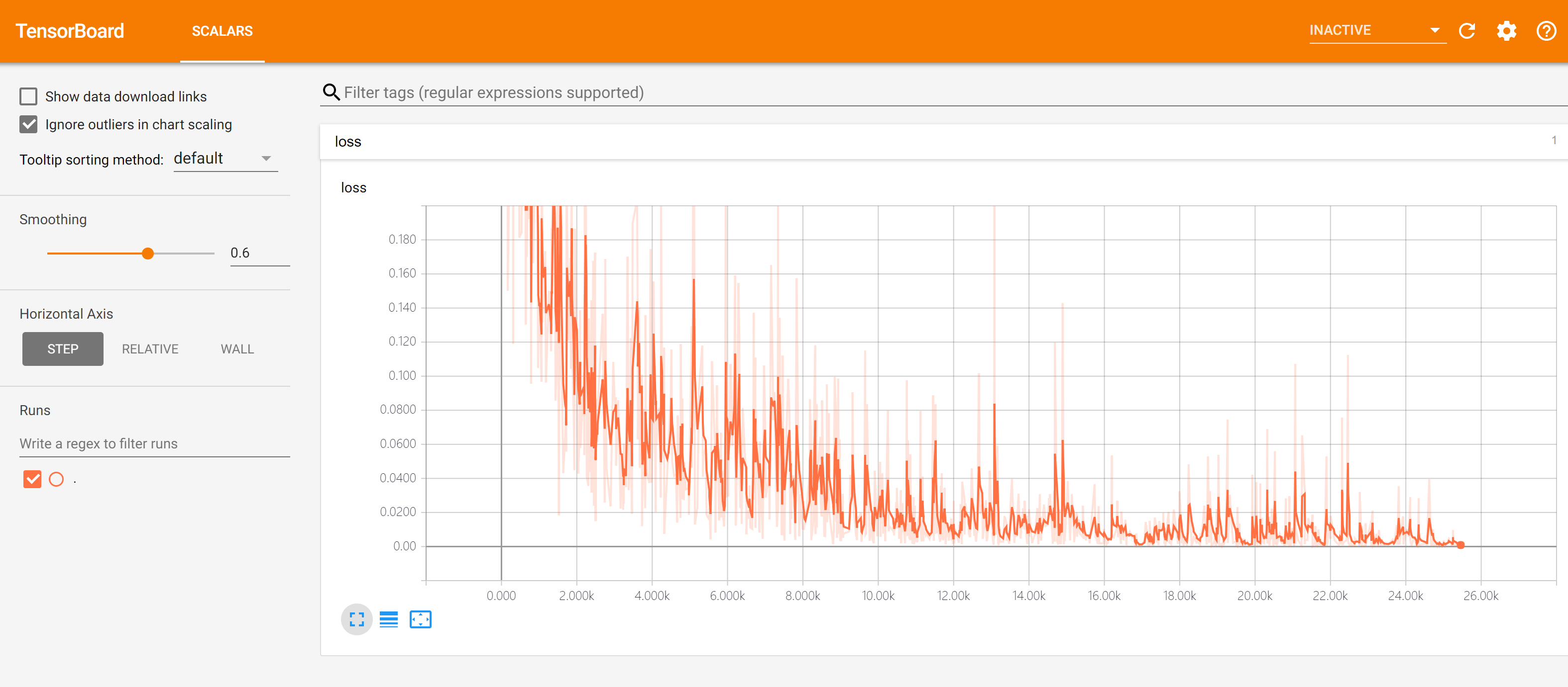
By default, TensorBoard updates data every 30 seconds. However, you can also manually refresh by clicking the refresh button in the upper right corner.
When using TensorBoard, please notice the following notes:
- If you want to retrain, you need to delete the information in the record folder and restart TensorBoard (or create a new record folder and open TensorBoard with the
--logdirparameter set to be the newly created folder); - Language of the record directory path should all be English.
Finally, we provide an example of the previous chapter’s multilayer perceptron model showing the use of TensorBoard:
import tensorflow as tf
import numpy as np
from en.model.mlp.mlp import MLP
from en.model.mlp.utils import DataLoader

tf.enable_eager_execution()
num_batches = 10000
batch_size = 50
learning_rate = 0.001
model = MLP()
data_loader = DataLoader()
optimizer = tf.train.AdamOptimizer(learning_rate=learning_rate)
summary_writer = tf.contrib.summary.create_file_writer('./tensorboard')     # instantiate a logger
with summary_writer.as_default(), tf.contrib.summary.always_record_summaries():
    for batch_index in range(num_batches):
        X, y = data_loader.get_batch(batch_size)
        with tf.GradientTape() as tape:
            y_logit_pred = model(tf.convert_to_tensor(X))
            loss = tf.losses.sparse_softmax_cross_entropy(labels=y, logits=y_logit_pred)
            print("batch %d: loss %f" % (batch_index, loss.numpy()))
            tf.contrib.summary.scalar("loss", loss, step=batch_index)       # log current loss
        grads = tape.gradient(loss, model.variables)
        optimizer.apply_gradients(grads_and_vars=zip(grads, model.variables))
GPU Usage and Allocation
Usually the scenario is: there are many students/researchers in the lab/company research group who need to use the GPU, but there is only one multi-card machine. At this time, you need to pay attention to how to allocate graphics resources.
The command nvidia-smi can view the existing GPU and the usage of the machine (in Windows, add C:\Program Files\NVIDIA Corporation\NVSMI to the environment variable “Path”, or in Windows 10 you can view the graphics card information using the Performance tab of the Task Manager).
Use the environment variable CUDA_VISIBLE_DEVICES to control the GPU used by the program. Assume that, on a four-card machine, GPUs 0, 1 are in use and GPUs 2, 3 are idle. Then type in the Linux terminal:
export CUDA_VISIBLE_DEVICES=2,3
or add this in the code,
import os
os.environ['CUDA_VISIBLE_DEVICES'] = "2,3"
to specify that the program runs only on GPUs 2, 3.
By default, TensorFlow will use almost all of the available graphic memory to avoid performance loss caused by memory fragmentation. You can set the strategy for TensorFlow to use graphic memory through the tf.ConfigProto class. The specific way is to instantiate a tf.ConfigProto class, set the parameters, and specify the “config” parameter when running tf.enable_eager_execution(). The following code use the allow_growth option to set TensorFlow to apply for memory space only when necessary:
config = tf.ConfigProto()
config.gpu_options.allow_growth = True
tf.enable_eager_execution(config=config)
The following code sets TensorFlow to consume 40% of GPU memory by the per_process_gpu_memory_fraction option:
config = tf.ConfigProto()
config.gpu_options.per_process_gpu_memory_fraction = 0.4
tf.enable_eager_execution(config=config)
Under “Graph Execution”, you can also pass the tf.ConfigPhoto class to set up when instantiating a new session.